SCaN – Reliability Assessment
Communication is Mission Critical
The NASA SCaN Network consists of many assets such as ground assets, in-space assets and even remote assets (e.g., mars rover), all organized under three divisions of SCaN: i) the Deep Space Network (DSN), ii) the Near Earth Network (NEN) and iii) the Space Network (SN). The technical objective of this effort was to demonstrate how PPI’s Technologies can be used to assess and quantify the reliability of NASA’s SCaN Network and to create a comprehensive capability for variety of issues including sensitivities, repair planning, resource allocation, etc.
Project Overview
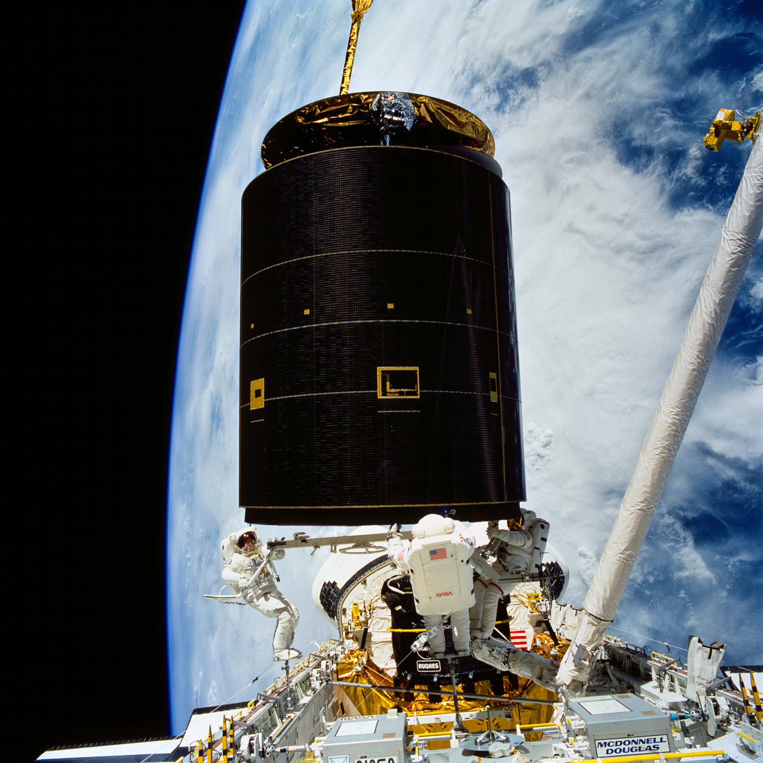
In this effort, PredictionProbe, Inc. (PPI) was contracted by the National Aeronautics and Space Administration (NASA) Glenn Research Center (GRC) to demonstrate capability and sample results for a combined probabilistic and Bayesian analysis reliability assessment of the NASA Space Communication and Navigation (SCaN) assets. The existing NASA SCaN network consists of many ground-based and space-based assets. The ground-based assets include many communication antennas of various diameters (up to 70 meters or about 230 feet), command centers, networks, controllers, data storage and data processing facilities. The space-based assets include a fleet of earth-orbiting NASA communications satellites. Beyond this, hundreds of national and international, commercial, and academic customers use the SCaN assets to transfer data to earth from their in-space and remote assets. As shown in Figure 1, the NASA SCaN assets are organized under three divisions: i) the Deep Space Network (DSN, see Figure 2), ii) the Near Earth Network (NEN, see Figure 3) and iii) the Space Network (SN, see Figure 4).
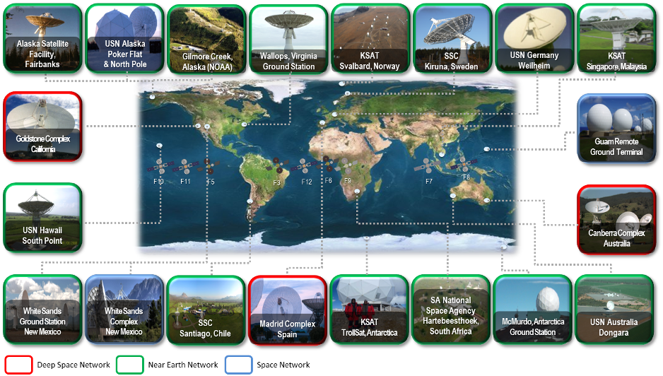
Figure 1.
The NASA Space Communication and Navigation Network
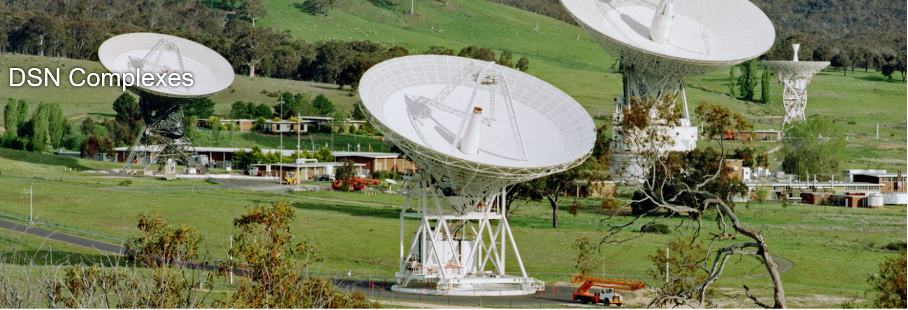
Figure 2.
Example of a NASA SCaN Deep Space Network (DSN) Complex.
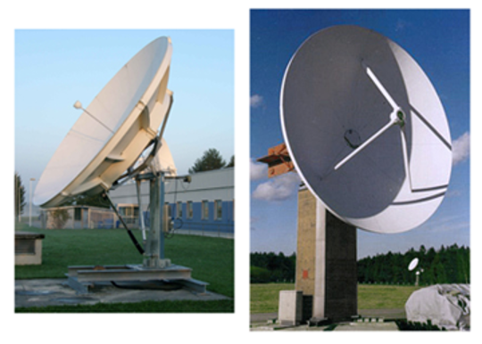
Figure 3.
Example of SCaN Near Earth Network (NEN) Complex.
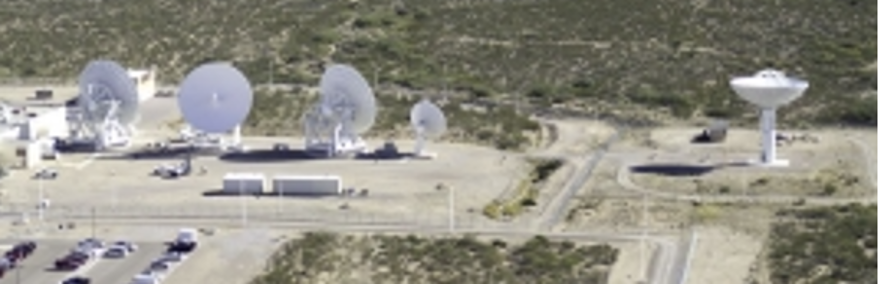
Figure 4.
Example of a NASA SCaN Space Network (SN) Complex.
Problem Definition
As noted above, the SCaN Network consists of many assets such as ground assets, in-space assets and even remote assets (e.g., mars rover), all organized under three divisions of SCaN: i) the Deep Space Network (DSN), ii) the Near Earth Network (NEN) and iii) the Space Network (SN). Each asset is comprised of one or more systems (antennae, power generation, power storage, networking, etc.) and numerous sub-systems (for example sub-systems within the antennae system include gimbal, ground structure, dish, etc.). Likewise, each sub-system may contain numerous components such as amplifiers, polarizers, and diplexers. The reliability of each component and sub-system affects the reliability of the system-level assets in which they are contained, and the reliability of each asset, in turn, influences the reliability of the SCaN network. While these assets, systems, sub-systems and components have each been designed to meet certain reliability levels, in practice however, the actual reliability of these systems and assets are uncertain due to numerous uncertainties such as physical damage, power outages or interruptions, environmental conditions, unforeseen usage scenarios, and so on.
This work was initiated to enable predictive computational capabilities for SCaN Networks to determine: 1) the impact of component reliabilities and failures, transmission latency, mission, orbital and location variables, uncertainties, etc. on network reliability; 2) the sensitivity of network reliability with respect to component reliability, latency, mission, orbital and location variables, uncertainties, etc.; 3) the consequences of a component failure in the network; 4) component time to failure, network availability; and 5) time to transmit data through the system. The technical objective of this effort was to demonstrate how PPI’s Technologies can be used to assess and quantify the reliability of NASA’s SCaN Network and to create a decision support capability to: 1) use Bayesian Technology to update input variable statistical models when additional data becomes available; 2) predict service reliability and its variation; 3) determine the impact of aging on service reliability; 4) perform parametric studies when adequate data is not available for proper modeling; 5) evaluate reliability of various communication configurations or architectures; 6) perform service repair planning; 7) determine sensitivity of service reliability to its components; 8) perform resource allocation using repair planning data; and 9) determine the costs associated with uncertainty. Please see the accompanying Case Studies on the SCaN Decision Support System and the Orion Reliability Assessment.
PredictionProbe’s Solution
Over the course of the project, several different demonstration problems were defined, analyzed, and delivered to the customer: 1) probabilistic reliability analysis (PRA) of a network with two assets; 2) Bayesian analysis of a network with 3 assets; 3) PRA of a Tracking and Data Relay Satellite; 4) PRA of two Goldstone Complex 34-meter antennas within the DSN; and 5) Bayesian updating of a selected input variable statistical model of the DSN demo problem. Numerous conclusions and recommendations from each demonstration were also provided in detail to the customer.
The First Demo Network consisted of a single ground station and a single satellite as shown below as a block diagram in Figure 5. The probabilistic reliability analysis of this network was performed using several workflows for the block diagram and its components. All reliability values and models were assumed by PPI. These workflows were constructed in SPISE® modeling environment. The results of this analysis were presented and explained to the customer during the kickoff meeting.
- Ground Station
- One Receiver with one Backup
- One Transmitter with one Backup
- One Power Supply with one Backup
- Satellite
- One Antenna
- One Antenna Controller
- One Receiver
- One Transmitter
- Solar Panel
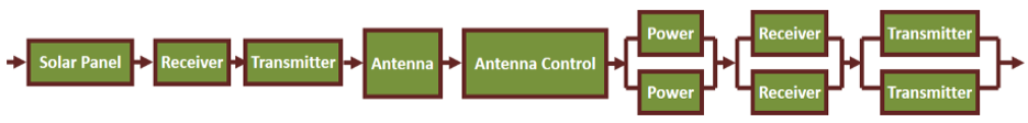
Figure 5.
Block Diagram for Probabilistic Reliability Analysis of The First Demo Network.
The Second Demo Network is depicted in Figure 6. The Probabilistic BBN of this system consisted of a generic model of the communication path between a rover with sensor (situated on Mars) and an Earth-based ground station. The communications path employed a single intermediate relay satellite between Mars and Earth, as shown in Figure 6. Algebraic reliability models (g1(x), g2(x), and g3(x)) were defined for each ground station, relay satellite and rover/sensor. Probabilistic uncertainty models were also defined as shown in Figure 6. These uncertainties cascade throughout the Bayesian Belief Network and predict the failure probability of the Second Demo Network.
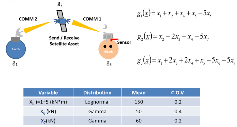
Figure 6.
The Second Demo Network.
The Third Demo Network was presented to the customer during a meeting at PPI’s headquarters in Newport Beach, California about two weeks after the project was formally started. This example consisted of detailed probabilistic reliability analysis for the hardware and services (see teal nodes) of a single tracking and data relay satellite (TDRS) satellite (TDRS-6, orange node) as shown in Figure 7.
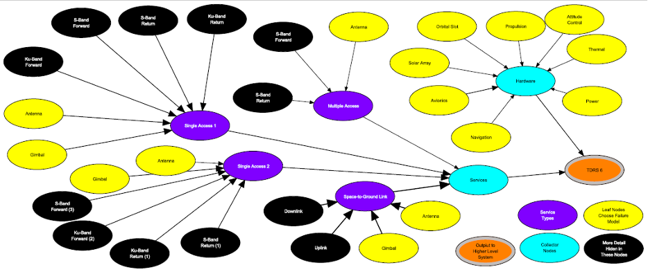
Figure 7.
Influence Diagram for TDRS-6, The Third Demo Network.
The hardware elements for this example included the following sub-systems, as defined by SCaN: Power, Thermal, Altitude Control, Propulsion, Orbital Slot, Solar Array, Avionics and Navigation (upper right yellow nodes). The services consist of the Space-to-Ground Link (STGL), two Single Access services (SA1 and SA2) and Multiple Access (MA), all shown as purple nodes in Figure 7. Each service includes a distinct on-board antenna (yellow nodes); all services except the MA also include an on-board gimbal (yellow nodes) to enable movement and pointing of the associated antenna. A top-level SPISE® workflow for this example is shown in Figure 8.
It is important to realize that only the highest-level detail about the reliability modeling is provided in Figure 7. The STGL service consists of an Uplink and Downlink. However, the Uplink includes the following hardware elements: power amplifier, diplexer and polarizer (all hidden inside of the black nodes in Figure 9); the Downlink includes the following hardware elements: low-noise amplifier, diplexer and polarizer (hidden). The remaining services SA1 and SA2 each consist of a Forward and Return link of various frequencies. Both the SA1 and SA2 services provide both S-Band and Ku-B and communications; each of these Forward links include the following hardware elements: power amplifier, diplexer and polarizer (hidden), while the Return links include the following hardware elements: low-noise amplifier, diplexer and polarizer (hidden). The MA service provides S-Band communications, similar to those described previously but without any diplexers involved. All of these hardware elements and services were defined by SCaN’s Team for PPI’s use and understanding.
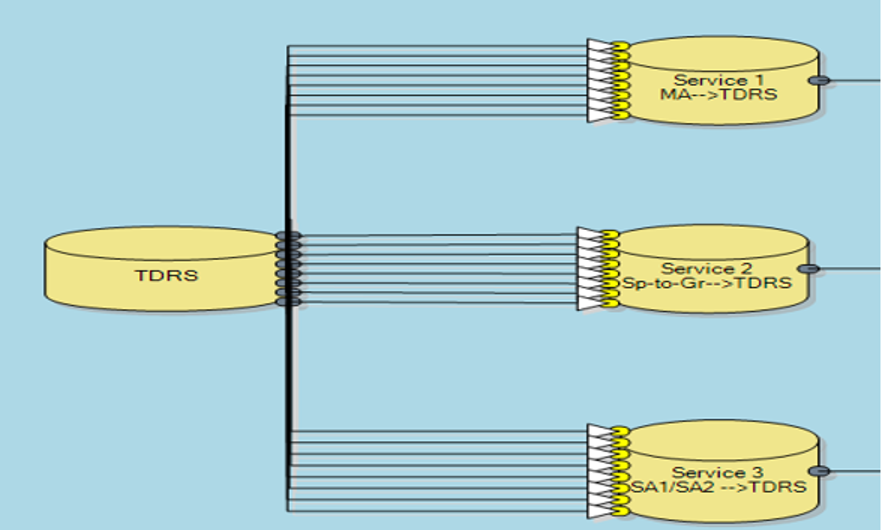
Figure 8.
Top-level SPISE Workflow for The Third Demo Problem.
The Fourth Demo Network was a very detailed, multi-faceted probabilistic reliability assessment of two 34-meter antennae (DSS-25 and DSS-26) within the SCaN / DSN Goldstone Complex. This demonstration was prepared for the customer within about four weeks of the project being initiated based upon considerable discussion between the customer and PPI. This example analyses and compares the reliability for seven services:
- Service 1 (S1): X-Band Downlink on DSS-25
- Service 2 (S2): Ka-Band Downlink on DSS-25
- Service 3 (S3): X-Band Uplink on DSS-25
- Service 4 (S4): Ka-Band Uplink on DSS-25
- Service 5 (S5): X-Band Downlink on DSS-26
- Service 6 (S6): Ka-Band Downlink on DSS-26
- Service 7 (S7): X-Band Uplink on DSS-26
A block diagram of the SPISE workflow for DSS-25 Downlink in this example is shown in Figure 9. The other workflows for this demonstration are similar, except that DSS-26 only offers X-Band Uplink.
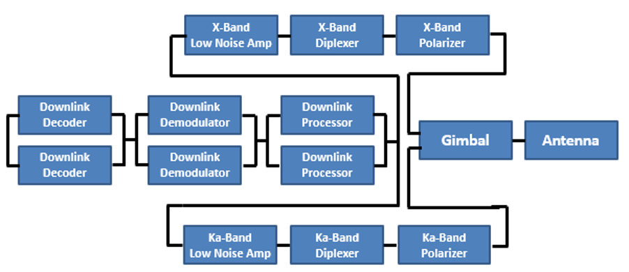
Figure 9.
Block Diagram of the DSS-25 Downlink Service from The Fourth Demo Problem.
The NASA customer required PPI to perform the following six analyses for the seven services:
- Downlink (Telemetry) Configurations:
- DSS-25 (X-Band) compared to DSS-26 (X-Band);
- DSS-25 (Ka-Band) compared to DSS-26 (Ka-Band);
- DSS-25 (X-Band) compared to DSS-26 (Ka-Band); and
- DSS-25 (Ka-Band) compared to DSS-26 (X-Band).
- Uplink (Command) Configurations:
- DSS-25 (X-Band) compared to DSS-26 (X-Band); and
- DSS-25 (Ka-Band) compared to DSS-26 (X-Band).
PPI planned, developed and executed the following analyses, all approved by NASA, in support of the NASA Requirements:
- Predict the variation of network reliability for one of the seven Services due to uncertainties associated with the reliabilities of its components;
- Estimate the network reliability for all seven Services;
- Estimate the network failure probability for a selected Service Configuration;
- Identify the sensitivity of the network reliability with respect to its hardware components for a selected Service;
- Provide capability to perform “what if” studies, such as adding or removing hardware, (e.g., providing or removing redundancies);
- Perform parametric studies when adequate data is not available;
- Predict aging effects on the network reliability due to aging of its hardware components based on simple aging models;
- Provide real-time network evaluation and trade study;
- Evaluate the seven network architectures defined by NASA;
- Demonstrate how to use of Probabilistic BBN in this demo problem; and
- Estimate the costs of the uncertainties (performed in Microsoft Excel).
All of the required input data were assumed by PPI and approved by NASA including:
- Component name;
- Component design life;
- Component usage per year (% of its design life);
- Component reliability reduction rate per year;
- Component minimum initial reliability; and
- Simplified aging models.
The Bayesian Analysis approach systematically incorporates subjective judgments based on intuition, experience, or indirect information with the observed data to obtain a balanced estimation of variable and predictive model parameters. Bayesian technologies include BBN, Probabilistic BBN, and Bayesian Updating Rule, all of which may be used for: updating variable models when new data becomes available; performing predictive model assessment, updating, and calibration; uncertainty-based decision making, and more.
Results & Conclusions
A sample execution of the baseline Probabilistic BBN for demo problem number two is illustrated in Figure 10. Given the definitions provided, the probability of failure (Pf) for the system (Pfsys) is less than 6%. As shown in Figure 11, the uncertainty models of the input variables for Probabilistic BBN has been updated, as a result of acquisition of new relevant data. Under these conditions, the probability of failure for the system rises to about 14%. The results of this analysis were presented and explained to the customer during the kickoff meeting.
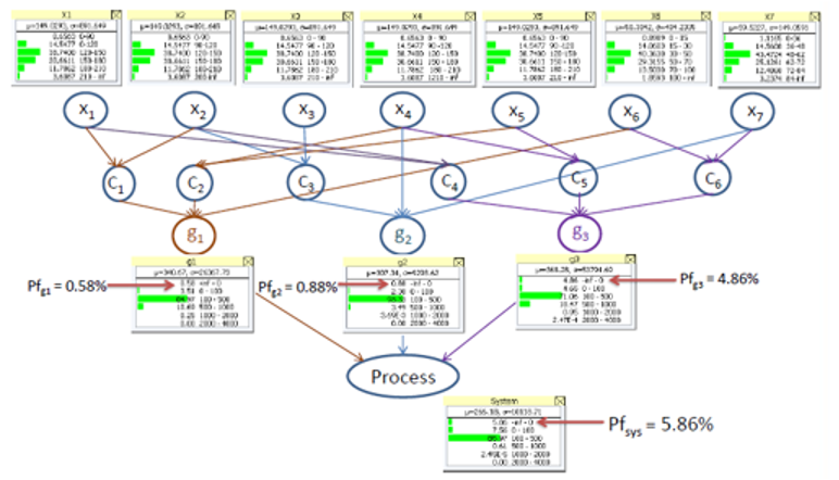
Figure 10.
Baseline Probabilstic BBN, Pfsys = 5.86%
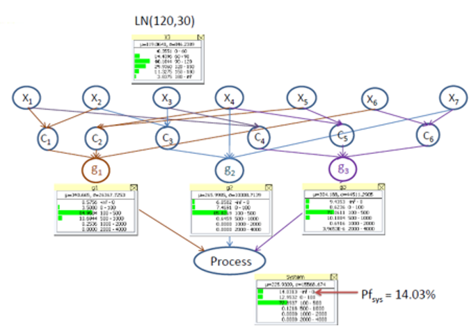
Figure 11.
Perturbed Probabilistic BBN, Pfsys = 14.03%
Sample executions of the SPISE workflows using assumed data for this problem were demonstrated for the customer. Typical execution sensitivity results are shown in Figures 12, respectively.
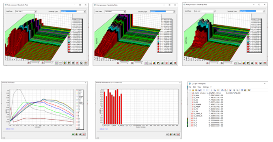
Figure 12.
Sample Top-Level Reliability Sensitivity Results for The Third Demo Network.
In the fourth demonstrational example, the seven services (Uplink and Downlink for Ka- and X-Band frequencies) associated with two 34-meter antennae were analyzed as follows: 1) estimated the network reliability for all seven services; 2) predicted the variation of network reliability due to the varying nature of component reliabilities; 3) estimated the network failure probability and its variation for a selected service configuration; 4) quantified the sensitivity of the network reliability with respect to the reliability of its hardware components for any service; 5) provided capability to perform “what if” studies, such as adding or removing hardware, (e.g., providing or removing redundancies); 6) performed parametric studies when adequate data is not available; 7) predicted aging effects on the network reliability based on simple component aging models that we assumed; 8) provided real-time network evaluation and trade study; 9) evaluated the seven network architectures defined by NASA; 10) demonstrated how to use Probabilistic BBN in this demo problem to update component life when new data become available; and 11) estimated the increase in maintenance cost due to the uncertainty of the component life. A second demonstration focused on the reliability assessment of a single Tracking and Data Relay (TDRS) satellite, with all communication services and sub-systems modeled. Sensitivity analysis was also performed to illustrate the changes in the overall TDRS reliability due to changes in the sub-system or service reliabilities.
In all cases, the required technologies and processes were fully demonstrated with representative network data due to the classified nature of the actual data. However, the applicability and success of PPI’s proposed approach is totally independent of whether or not the data used is representative or actual.
Figure 13 illustrates the typical variability of sample results for S1; shown in the Figure are the probability density function (PDF) and the cumulative distribution function (CDF) of the S1 reliability. Due to uncertainties and naturally occurring variabilities, the reliability of S1 is not a single number, but rather, a distribution of numbers. Subsequent results reference five specific points of these distributions: 1%, 10%, 50%, 90% and 99%, which are highlighted in red in the bottom portion of Figure 13.
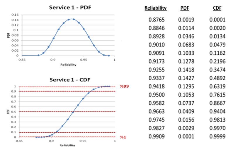
Figure 13.
Sample Reliability Results from The Fourth Demo Network.
Typical aging results over time are shown in Figure 14, again for S1. Again, the reliability of a given component of time is not a single number or even a single curve, but rather a set of distributions, as shown in Figure 14. A replacement of worn parts procedure was proposed to the customer based upon the predicted time in years at which a certain point of the distribution crosses below a pre-agreed upon reliability level. For example, the lowest curve in Figure 14 (1% of the reliability distribution) crosses through 80% reliability at just less than 4 years of service time, as indicated by the red arrows in Figure 14. This information could be used to plan maintenance and replacement of parts. A comparison of the reliability of various services over time is shown in Figure 15. The four Downlink services all exhibit much lower reliability over time than do the X-Band Uplink services. Sample system reliability sensitivity results are shown in Figure 16. Under the assumptions made, the system reliability exhibits the greatest sensitivity (tallest bars in the bar chart) to the antenna, gimbal, and amplifier/diplexer, respectively. The antenna and gimbal are quite expensive and also intended to have a long lifespan. However, the amplifier and diplexer would likely need to be replaced using a maintenance scheme such as that proposed above.
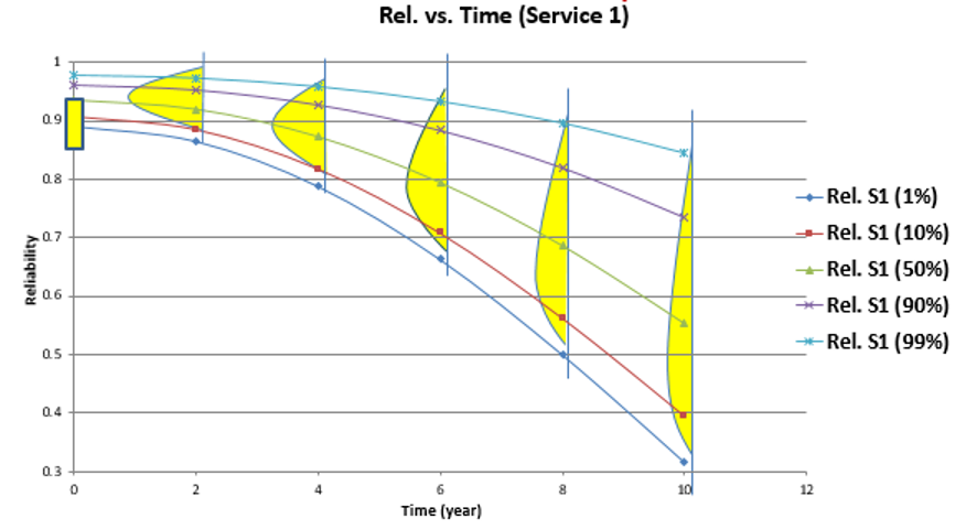
Figure 14.
Sample Aging Results from The Fourth Demo Network.
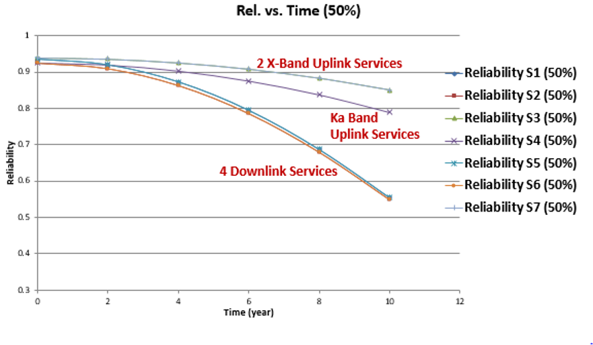
Figure 15.
Sample Aging Comparison from The Fourth Demo Network.
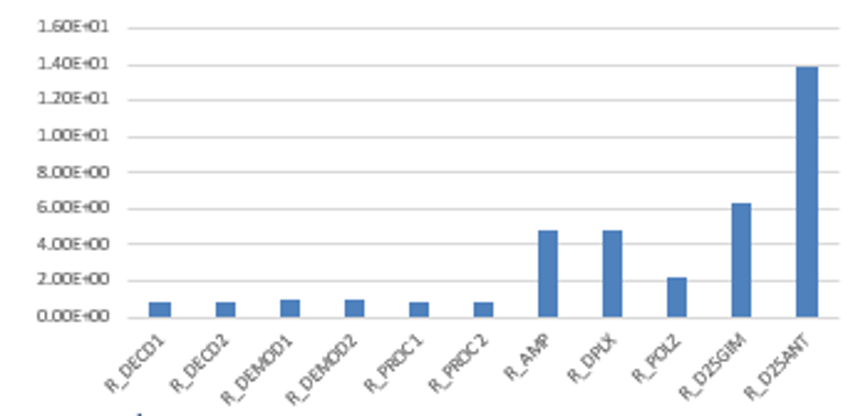
Figure 16.
Sample Reliability Sensitivity Results from The Fourth Demo Network.
About PredictionProbe, Inc.
PredictionProbe, Inc. is a small business and proud provider of an elite offering of world-class predictive technologies, tools, and services that enable decision makers with real solutions for real world challenges. To learn more visit us at: predictionprobe.com
PredictionProbe, Inc. ©2020. All rights reserved.